Camera Calibration 相机标定：原理简介（四）

4 基于3D标定物的标定方法

使用基于3D标定物进行相机标定，是一种传统且常见的相机标定法。3D标定物在不同应用场景下不尽相同，摄影测量学中，使用的3D标定物种类最为繁杂，如图-1的室内控制场，由多条悬垂的杆组成，杆与墙壁不同位置上贴着标志点，并通过精密测量的方法，获得标志点的三维坐标，精度较高，但成本极其昂贵，而且需要定期维护，一般个人或实验室请慎入！计算机视觉中，经典的两种3D标定物，如图-2所示，图-2(a)是INRIA(1993)所使用的，由两个正交的平面组成，棋盘方形格图案被绘制在每个面上，并且提供其中角点的精确坐标；类似的还有用立方体（Cube），每个面同样也绘制上相同图案，相机可以对其三个面进行成像；另外还有非常流行的 Tsai(1987)所提出的标定设备和方法，如图-2(b)，只使用与图-2(a)中相同的一个平面，但是在使用时，需要至少将标定平面移动一次位置，且移动信息是明确已知的。

图-1 摄影测量室内控制场

图-2 两种3D标定物

图-3 法国INRIA

4.1 主要流程

这一类标定法，主要包括四个步骤：

1. 检测每张图片中的棋盘图案的角点（Detect the corners of the checker pattern in each image）；

2. 通过使用线性最小二乘法估算相机投影矩阵P（Estimate the camera projection matrix P using linear least squares）；

3. 根据P矩阵求解内参矩阵和外参A,R和t（Recover intrinsic and extrinsic parameters A,R and t from P）；

4. 通过非线性优化，提高A,R和t矩阵的精度（Refine A,R and t through a nonlinear optimization）。

除了上述的流程，还有另外一种做法是先通过非线性优化改善相机投影矩阵P，然后获得相机内参和外参。

4.2 角点检测

一般来说，为了提高角点检测的准确度和精度，标定板图案中会使控制点处的梯度或对比反差最大化。即便如此，使用普通的角点检测方法，例如Harris，提取图像中的角点，往往难以获得较好的精度（超过一个像素）。

较好的解决手段是，事先知道图案结构的情形下，提取出各个矩形框的边，然后通过边所在直线相交的方法获得角点。例如常见的两种方法：第一种，首先进行边缘检测，将各个矩形框边缘拟合成直线；第二种，直接根据梯度最大原则，从矩形框的每一边拟合出直线。如果不考虑镜头畸变（ lens distortion）更好的做法是，将共线的矩形框边缘，拟合成为一条直线，然后再求得交点。

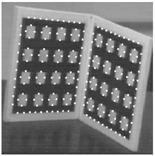
图-4 一种基于最大梯度的角点检测结果

4.3 线性估算相机投影矩阵

一旦我们提取出图像中的角点，根据先验知识（图案的结构特点）就可以比较轻易的将这些角点与其对应的物方点相对应。根据原理简介（二）中的投影方程，我们就可以估算相机参数。但是问题是，直接求解A,R和t由于属于非线性问题，因而并不能实现。而通过线性估算投影矩阵P是可以实现的。

给定一组2D-3D对应点对：mi=(ui,vi)↔Mi=(Xi,Yi,Zi)，则有：

其中，p=[p11,p12,…,p34]T,0=[0,0]T，令p矩阵的系数矩阵简记为Gi。对于n个点对，我们将其组成一个方程组：

可知，G是一个2n×12的矩阵。于是投影矩阵能够通过公式(3)的约束获得：

这一解法目的就是要使特征向量GTG所对应的特征值最小化。同时为了避免平凡解（ trivial solution）p=0和考虑到实际情况，p形似一个尺度系数，此处设其模长为1。

上述的线性解法，实质上是一个代数距离最小化的方法，也就是耳熟能详的最小二乘法（Least squares），当数据存在偏差或噪声时，就会导致估算结果偏差，后续将会介绍一种无偏求解的方法。

4.4 根据P获取内参和外参

由前文的分析知，P是3×4的矩阵，如果我们将其分成两块：前三列（3×3）的矩阵B和最后一列（3×1）的矩阵b，因此矩阵P可以表示为：P≡[B  b]，又知道P=A[R  t]，则有：

由公式(4)可以推出：

由于，令ku=α2+γ2+u20，kc=u0v0+γβ，kv=β2+v20。前文已经提到，P形似一个尺度系数，实际中，K矩阵的最后一个元素K33≠1，因此需要对其进行归一化，之后就可以获得内参：

由于α>0,β>0所以上述参数的解是唯一的。而内参获得后，相应的内参矩阵也就获得，外参矩阵自然也就可以解出：

4.5 非线性优化标定参数

上面获得相机内参和外参的方法，仅仅是依据代数距离最小约束，并不能完全代表物理含义，也就是说，获得的解是有偏差的。可以通过最大似然法（Maximum likelihood）提高解的精度。

给定n组2D-3D点对：mi=(ui,vi)↔Mi=(Xi,Yi,Zi)，假设像点精度的受一系列不相关且独立分布的噪声影响，最大似然法通过使观测像点与其通过成像模型预测的像点之间的差异最小化，对模型参数进行优化：

其中，ϕ(P,Mi)是通过相机投影模型得到的像点。这个优化问题，属于非线性问题，可以利用著名的LM算法（Levenberg-Marquardt Algorithm）解决。

4.6 镜头畸变

行文至此，我们已经对针孔相机有了些许了解，我们利用成像的过程中三维空间点，相机光学中心和像点之间的共线性，得到成像方程。但是这一线性投影方程并不一定对所有针孔相机都适用，尤其是一些低端相机和广角相机，这些相机的镜头畸变往往较大，对之不能置之不理。

解决镜头畸变同样也需要四步：

• 刚体变换（Rigid transformation）：从物空间坐标系(X,Y,Z)到像空间坐标系(x,y,z)：

• 透视投影（Perspective projection）：从像空间坐标系到理想的像平面坐标系(x′,y′)，也就是说不考虑镜头畸变时的像平面坐标：

• 镜头畸变（Lens distortion）：对于未考虑镜头畸变的像点，对其补偿畸变值后，即可得到畸变纠正后的像点(x^,y^)：

• 仿射变换（Affine transformation）：将以相片中心为坐标系的坐标变换到以像素为单位的图像坐标(u^,v^)：
  u^=d−1xx^+u0,  v^=d−1yy^+v0(18)

  其中，(u0,v0)是像主点，(dx,dy)分别是像素水平方向和垂直方向的物理尺寸。

研究表明，镜头畸变主要分为两种：

• 径向畸变（Radial distortion）：使得成像点沿着向径方向（像主点与像点之间的连线方向）偏离其准确理想的位置，根据畸变系数的正负，又可以分为桶形畸变和枕形畸变两种。

• 偏心畸变（Decentering distortion）：常由镜头安装不当导致，偏心畸变差引起径向和切向的像点位移，偏心畸变一般来说只有径向畸变的1/7∼1/8，因此有些简化分析模型会将其忽略。

令r=x′2+y′2−−−−−−−√，则畸变模型为：

其中，ki是径向畸变系数，pi是偏心畸变系数。如果仅仅考虑径向畸变，且令u=x′/dx,  v=y′/dy则，像点坐标(u^,v^)可以表示为：

将畸变考虑到非线性优化公式(14)中：

其中，m^(A,R,t,k1,k2,Mi)是物方点Mi在图像上的投影像点。